The Time History Analysis add-on provides you with accelerograms for the calculation. This extension allows for dynamic structural analysis of the acceleration-time diagrams.
There is an extensive library of earthquake records available for you, but you can also enter or import your own diagrams. The time history analysis is performed using the modal analysis or the linear implicit Newmark analysis.
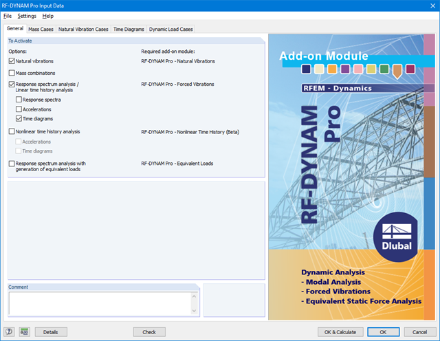
- Analysis of time diagrams and accelerograms (acceleration-time diagrams exciting the supports of a structure)
- Combination of user-defined time diagrams with nodal, member, and surface loads, as well as free and generated loads
- Combination of several independent excitation functions
- Linear implicit Newmark analysis or modal analysis in time history
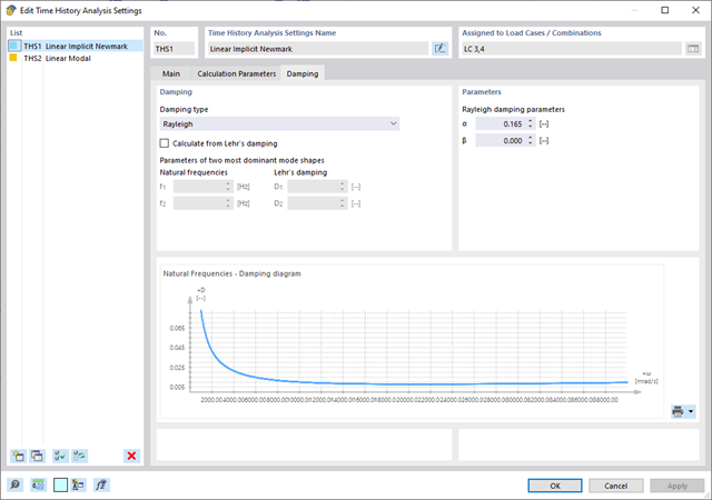
- Structural damping using Raleigh damping coefficients or Lehr's damping value
- Graphical display of results in calculation diagrams
- Result display in individual time steps or as an envelope during the entire time period
- Extensive library of seismic events (accelerograms)
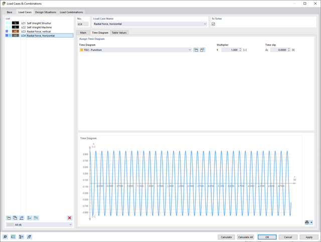
It is necessary to enter the required force-time diagrams. They can be combined in load cases or load combinations of the type Time History Analysis | Time Diagrams with the loading in order to define where and in which direction the force-time diagrams act.
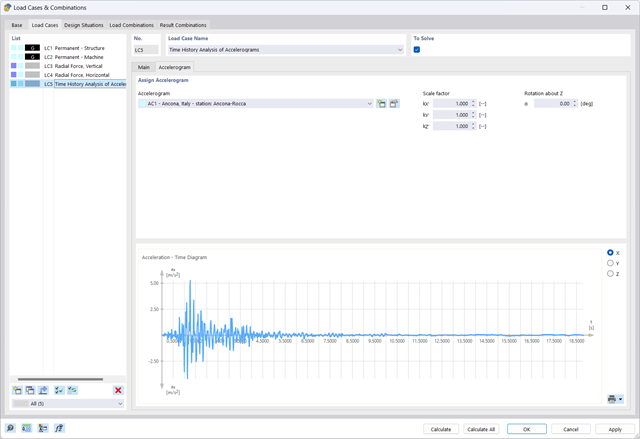
The second option is to enter acceleration-time diagrams, which can be used in the load cases of the Time History Analysis | Accelerogram type.
All calculation parameters are specified in the time history analysis settings. These include, for example, the type of analysis method and the maximum calculation time.
During the calculation, the selected horizontal load is increased in load steps. A static nonlinear analysis is carried out for each load step until reaching the specified limit condition.
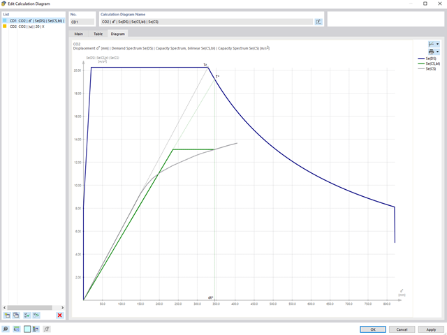
The results of the pushover analysis are extensive. On one hand, the structure is analyzed for its deformation behavior. This can be represented by a force-deformation line of the system (a capacity curve). On the other hand, the response spectrum effect can be displayed in the ADRS display (Acceleration-Displacement Response Spectrum). The target displacement is automatically determined in the program based on these two results. The process can be evaluated graphically and in tables.
The individual acceptance criteria can then be graphically evaluated and assessed (for the next load step of the target displacement, but also for all other load steps). The results of the static analysis are also available for the individual load steps.

The Dlubal structural analysis software does a lot of work for you. The input parameters, which are relevant for the selected standards, are suggested by the program in accordance with the rules. Furthermore, you can enter response spectra manually.
Load cases of the type Response Spectrum Analysis define the direction in which response spectra act and which eigenvalues of the structure are relevant for the analysis. In the spectral analysis settings, you can define details for the combination rules, damping (if applicable), and zero-period acceleration (ZPA).
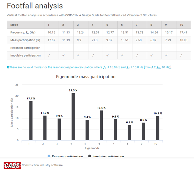
- Overall maximum response factors and critical nodes
- Resonant analysis (maximum response factor, RMS acceleration, critical node, critical frequency)
- Impulsive (transient) analysis (maximum response factor, peak acceleration/velocity, RMS acceleration/velocity, critical node, critical frequency)
- Vibration dose values for both resonant and impulsive analyses
Charts
- Response factor vs walking frequency
- Mass participation vs eigenmodes
- Velocity time history
It is necessary to enter the required response spectra, accelerations, or time diagrams. Dynamic load cases define the location and direction of response spectra effects as well as acceleration time, or force-time excitations.
Timing diagrams are combined with static load cases, which provides great flexibility. For the time history analysis, you can import the initial deformation from any load case or load combination.
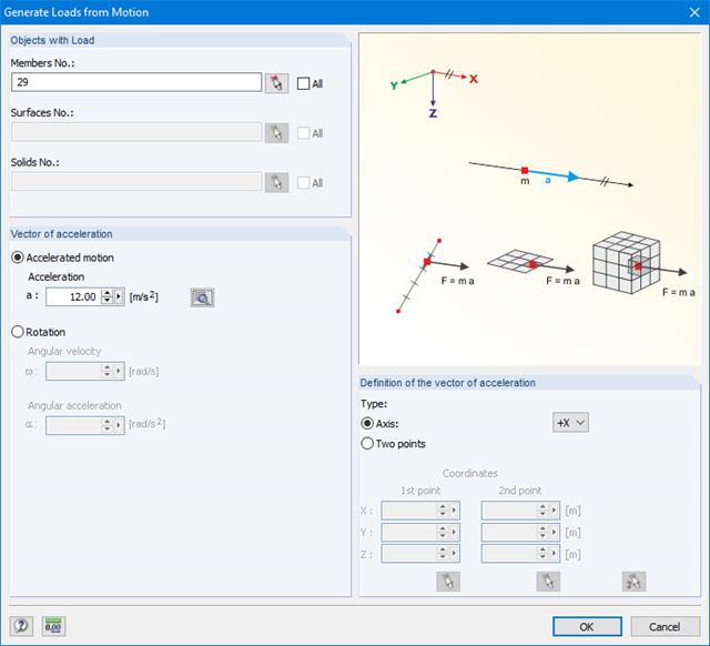
This generator creates loads as a result of an acceleration or rotation (e.g. from tower cranes), which acts on specific objects of the model.
The mass is determined from the self-weight.
More Information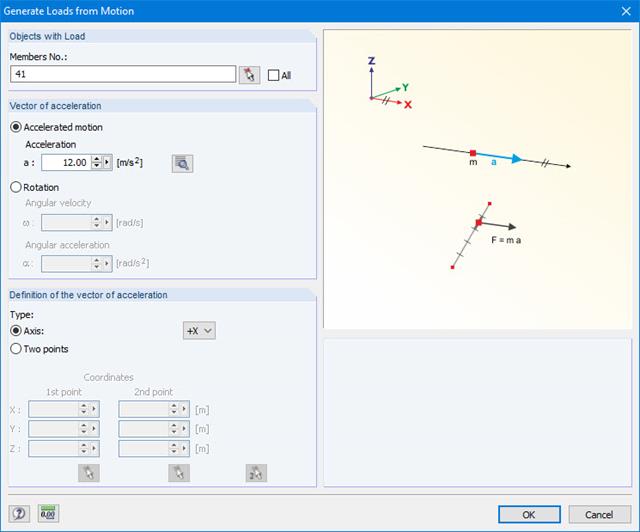
This generator creates loads as a result of an acceleration or rotation that acts on specific objects of the model.
The mass is determined from the self-weight.
More Information